I’ve been spending some time thinking about spinors on curved spacetime. There exists a decent set of literature out there for this, but unfortunately it’s scattered across different `cultures’ like a mathematical Tower of Babel. Mathematicians, general relativists, string theorists, and particle physicists all have a different set of tools and language to deal with spinors.
Particle physicists — the community from which I hail — are the most recent to use curved-space spinors in mainstream work. It was only a decade ago that the Randall-Sundrum model for a warped extra dimension was first presented in which the Standard Model was confined to a (3+1)-brane in a 5D Anti-deSitter spacetime. Shortly after, flavor constraints led physicists to start placing fields in the bulk of the RS space. Grossman and Neubert were among the first to show how to place fermion fields in the bulk. The fancy new piece of machinery (by then an old hat for string theorists and a really old hat for relativists) was the spin connection which allows us to connect the flat-space formalism for spinors to curved spaces. [I should make an apology: supergravity has made use of this formalism for some time now, but I unabashedly classify supergravitists as effective string theorists for the sake of argument.]
One way of looking at the formalism is that spinors live in the tangent space of a manifold. By definition this space is flat, and we may work with spinors as in Minkowski space. The only problem is that one then wants to relate the tangent space at one spacetime point to neighboring points. For this one needs a new kind of covariant derivative (i.e. a new connection) that will translate tangent space spinor indices at one point of spacetime to another.
By the way, now is a fair place to state that mathematicians are likely to be nauseous at my “physicist” language… it’s rather likely that my statements will be mathematically ambiguous or even incorrect. Fair warning.
Mathematicians will use words like the “square root of a principle fiber bundle” or “repere mobile” (moving frame) to refer to this formalism in differential geometry. Relativists and string theorists may use words like “tetrad” or “vielbein,” the latter of which has been adopted by particle physicists.
A truly well-written “for physicists” exposition on spinors can be found in Green, Schwartz, and Witten, volume II section 12.1. It’s a short section that you can read independently of the rest of the book. I will summarize their treatment in what follows.
We would like to introduce the a basis of orthonormal vectors at each point in spacetime,  , which we call the vielbein. This translates to `many legs’ in German. One will often also hear the term vierbein meaning `four legs,’ or `funfbein’ meaning `five legs’ depending on what dimensionality of spacetime one is working with. The index
  refers to indices on the spacetime manifold (which is curved in general), while the index
  labels the different basis vectors.
If this makes sense, go ahead and skip this paragraph. Otherwise, let me add a few words. Imagine the tangent space of a manifold. We’d like a set of basis vectors for this tangent space. Of course, whatever basis we’re using for the manifold induces a basis on the tangent space, but let’s be more general. Let us write down an arbitrary basis. Each basis vector has  components, where is the dimensionality of the manifold. Thus each basis vector gets an undex from 1 to , which we call
  . The choice of this label is intentional, the components of this basis map directly (say, by exponentiation) to the manifold itself, so these really are indices relative to the basis on the manifold. We can thus write a particular basis vector of the tangent space at
  as
as  . How many basis vectors are there for the tangent space? There are . We can thus label the different basis vectors with another letter, . Hence we may write our vector as .
The point, now, is that these objects allow us to convert from manifold coordinates to tangent space coordinates. (Tautological sanity check: the are tangent space coordinates because they label a basis for the tangent space.) In particular, we can go from the curved-space indices of a warped spacetime to flat-space indices that spinors understand. The choice of an orthonormal basis of tangent vectors means that
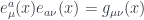 ,
,
where the index is raised and lowered with the flat space (Minkowski) metric. In this sense the vielbeins can be thought of as `square roots’ of the metric that relate flat and curved coordinates. (Aside: this was the first thing I ever learned at a group meeting as a grad student.)
Now here’s the good stuff: there’s nothing `holy’ about a particular orientation of the vielbein at a particular point of spacetime. We could have arbitrarily defined the tangent space z-direction (i.e.  , not $\mu=3$) pointing in one direction (
 ) or another (
 ) relative to the manifold’s basis so long as the two directions are related by a Lorentz transformation. Thus we have an
  symmetry (or whatever symmetry applies to the manifold). Further, we could have made this arbitrary choice independently for each point in spacetime. This means that the symmetry is local, i.e. it is a gauge symmetry. Indeed, think back to handy definitions of gauge symmetries in QFT: this is an overall redundancy in how we describe our system, it’s a `non-physical’ degree of freedom that needs to be `modded out’ when describing physical dynamics.
Like any other gauge symmetry, we are required to introduce a gauge field for the Lorentz group, which we shall call  . From the point of view of Riemannian geometry this is just the connection, so we can alternately call this creature the spin connection. Note that this is all different from the (local) diffeomorphism symmetry of general relativity, for which we have the Christoffel connection.
What do we know about the spin connection? If we want to be consistent with general relativity while adding only minimal structure (which GSW notes is not always the case), we need to impose consistency when we take covariant derivatives. In particular, any vector field with manifold indices ( ) can now be recast as a vector field with tangent-space indices (
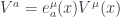 ). By requiring that both objects have the same covariant derivative, we get the constraint
 .
.
Note that the covariant derivative is defined as usual for multi-index objects: a partial derivative followed by a connection term for each index. For the manifold index there’s a Christoffel connection, while for the tangent space index there’s a spin connection:
 .
.
This turns out to give just enough information to constrain the spin connection in terms of the vielbeins,
![\omega^{ab}_\mu = \frac 12 g^{\rho\nu}e^{[a}_{\phantom{a}\rho}\partial_{\nu}e^{b]}_{\phantom{b]}\nu}+ \frac 14 g^{\rho\nu}g^{\tau\sigma}e^{[a}_{\phantom{[a}\rho}e^{b]}_{\phantom{b]}\tau}\partial_{[\sigma}e^c_{\phantom{c}\nu]}e^d_\mu\eta_{cd}](https://s0.wp.com/latex.php?latex=%5Comega%5E%7Bab%7D_%5Cmu+%3D+%5Cfrac+12+g%5E%7B%5Crho%5Cnu%7De%5E%7B%5Ba%7D_%7B%5Cphantom%7Ba%7D%5Crho%7D%5Cpartial_%7B%5Cnu%7De%5E%7Bb%5D%7D_%7B%5Cphantom%7Bb%5D%7D%5Cnu%7D%2B+%5Cfrac+14+g%5E%7B%5Crho%5Cnu%7Dg%5E%7B%5Ctau%5Csigma%7De%5E%7B%5Ba%7D_%7B%5Cphantom%7B%5Ba%7D%5Crho%7De%5E%7Bb%5D%7D_%7B%5Cphantom%7Bb%5D%7D%5Ctau%7D%5Cpartial_%7B%5B%5Csigma%7De%5Ec_%7B%5Cphantom%7Bc%7D%5Cnu%5D%7De%5Ed_%5Cmu%5Ceta_%7Bcd%7D&bg=ffffff&fg=29303b&s=0&c=20201002) ,
,
this is precisely equation (11) of hep-ph/980547 (EFT for a 3-Brane Universe, by Sundrum) and equation ( 4.28 ) of hep-ph/0510275 (TASI Lectures on EWSB from XD, Csaki, Hubisz, Meade). I recommend both references for RS model-building, but note that neither of them actually explain where this equation comes from (well, the latter cites the former)… so I thought it’d be worth explaining this explicitly. GSW makes a further note that the spin connection can be using the torsion since they are the only terms that survive the antisymmetry of the torsion tensor.
Going back to our original goal of putting fermions on a curved spacetime, in order to define a Clifford algebra on such a spacetime it is now sufficient to consider objects 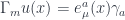 , where the right-hand side contains a flat-space (constant) gamma matrix with its index converted to a spacetime index via the position-dependent vielbein, resulting in a spacetime gamma matrix that is also position dependent (left-hand side). One can see that indeed the spacetime gamma matrices satisfy the Clifford algebra with the curved space metric,
 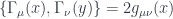 .
.
There’s one last elegant thought I wanted to convey from GSW. In a previous post we mentioned the role of topology on the existence of the (quantum mechanical) spin representation of the Lorentz group. Now, once again, topology becomes relevant when dealing with the spin connection. When we wrote down our vielbeins we assumed that it was possible to form a basis of orthonormal vectors on our spacetime. A sensible question to ask is whether this is actually valid globally (rather than just locally). The answer, in general, is no. One simply has to consider the “hairy ball” theorem that states that one cannot have a continuous nowhere-vanishing vector field on the 2-sphere. Thus one cannot always have a nowhere-vanishing global vielbein.
Topologies that can be covered by a single vielbein are actually `comparatively scarce’ and are known as parallelizable manifolds. For non-parallelizable manifolds, the best we can do is to define vielbeins on local regions and patch them together via Lorentz transformations (`transition functions’) along their boundary. Consistency requires that in a region with three overlapping patches, the transition from patch 1 to 2, 2 to 3, and then from 3 to 1 is the identity. This is indeed the case.
Spinors must also be patched together along the manifold in a similar way, but we run into problems. The consistency condition on a triple-overlap region is no longer always true since the double-valuedness of the spinor transformation (i.e. the spinor transformation has a sign ambiguity relative to the vector transformation). If it is possible to choose signs on the spinor transformations such that the consistency condition always holds, then the manifold is known as a spin manifold and is said to admit a spin structure. In order to have a consistent theory with fermions, it is necessary to restrict to a spin manifold.


 theory or massless QCD. We shall further restrict to dimensionless observables, such as the ratio of cross sections. Let’s call a general observable
  , where we have inserted a dependence on the energy
  with foresight that such things renormalize with energy scale.
 which depends only on two massive variables
  and which is
 only,
only,  .
. , then
  ,
, is the usual beta function calculated in perturbation theory. It is dimensionless and is uniquely defined by the theory. Another way one can define
  constant
 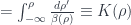 .
. ,
, we see that
  . Thus we see finally that the integral of the
  .
. is an integral that comes from the
  vanishes for some
  , then we can write our observable in terms of this scale,
 .
. is fixed for a particular theory. This latter quantity is rather interesting because even though it is an intrinsic property of the black box, it is not predicted by the black box, it must be fixed by explicit measurement of an observable.
 .
. and the field strength renormalization
  are also formally divergent, but in a way that cancels the divergence of the bare field and couplings.
 -matrices in some representation, one can work with
  -matrices (Pauli matrices) which have a single standard representation. The “gamma gymnastics” of calculations thus becomes simpler.
 ) live in different representations of the SM gauge group. This poses a rather rigid constraint on what kind of model becomes effective at the TeV scale.
 ), since this means one would be able to take a spin +1/2 fermion
  and expect to find a spin -1/2 fermion
  in the same supermultiplet (i.e. with the same gauge quantum numbers).
 rotation does not return them to their initial state, but a
  relation does. (For a classical analogue, see Bolker’s
  . This is a complex number that can be decomposed into an magnitude and a phase. Physical observables, however, are given only by the magnitude of the wavefunction and are independent of the phase. Relative phases can, of course, produce physical effects; but we’re focusing on one-particle states.
 are represented by matrices
  with the property (by the definition of a representation) that
 .
. such that
 .
. we work with the simply connected group
  . The fundamental representations are the very Weyl spinors that we know and love.